Caleb K. Harada
Astrophysics Ph.D. Candidate
University of California, Berkeley
Hello! I'm an Astrophysics Ph.D. Candidate and National Science Foundation Graduate Research Fellow at UC Berkeley. Prior to grad school, I completed my undergraduate education at the University of Maryland, College Park, where I studied astronomy and physics. My research interests broadly include the detection and characterization of planets orbiting stars beyond the Solar System, known as exoplanets. I'm especially curious about what observations and theory of extra-solar systems can teach us about our own solar system, how we got here, and whether we are alone in the universe (see research highlights). Beyond research, I'm passionate about making science more inclusive and accessible through teaching, mentoring, outreach, and community building. When I'm not thinking about science, I love to hike, go birdwatching, admire my cat, and explore the fresh produce selection at Berkeley Bowl. I use they/them pronouns.
Read my CV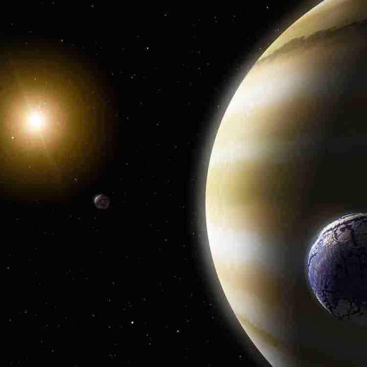
As remnants of star formation, planets help tell the story of how solar systems like ours form and evolve over their lifetimes. Observations of planets both in our solar system and beyond demonstrate an incredible diversity of possible planet formation outcomes and a staggering abundance of exoplanets spanning orders of magnitude in mass, radius, temperature, and age. Their orbital characteristics, atmospheric and interior compositions and structures, host star properties, system architectures, and cosmic birth environments are just as impressively varied. And of course, planets are the only objects in the universe known so far to support life. However, the census of exoplanets is still largely incomplete and the field is ripe for new discovery. Decades of scientific progress has led us to the precipice of addressing some of humanity's most fundamental questions: Just how special is our home world and our solar system? And are we alone?
Research Highlights
I'm a big fan of open-source software. My research wouldn't be possible without it! I enjoy developing open-source tools that are useful to the exoplanet and broader astronomical communities. Here are a couple of documented, pip-installable Python packages I've created. More to come soon!
Learn more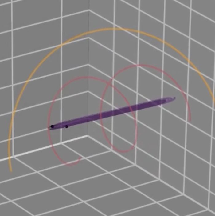
I love turning complex ideas into things that people can see and feel. This page contains a few pedagogical demos that I created as side projects or class assignments over the years. I think they're pretty neat and worth sharing. Feel free to use them as teaching tools in your next lecture (and please give me credit if you do!). Enjoy!
View demosDo not undertake a scientific career in quest of fame or money. There are easier and better ways to reach them. Undertake it only if nothing else will satisfy you; for nothing else is probably what you will receive. Your reward will be the widening of the horizon as you climb. And if you achieve that reward you will ask no other.
— Cecilia Payne-Gaposchkin, An Autobiography and Other Recollections (1984)
Innumerable celestial bodies, stars, suns and earths may be sensibly perceived...by us, and an infinite number of them may be inferred by our own reason. [A]ll those worlds...contain animals and inhabitants no less than can our own earth, since those worlds have no less virtue nor a nature different from that of our earth.
— Giordano Bruno, De l'Infinito, Universo e Mondi (1584)