The Sloan Digital Sky Survey (SDSS) represents the state-of-the-art for a deep, wide field optical survey (g' = 22.2 AB 10-sigma / 10,000 sq. degrees / 0.4-0.9 micron). Near-IR surveys, such as 2MASS, have had tremendous impact, but their sensitivity (K=15.8 AB 10-sigma) is limited by intense air glow, and an equivalent near-IR survey is impossible from the ground. However, from space a survey which is ~ 10 mag deeper than 2MASS is feasible. To maximise the scientific return from major facilities, especially NGST, deeper wide-field surveys over more extended wavelength ranges, particularly the near-IR, are a pre-requisite. We propose a near-IR survey to address three major components of NASA Origin's program: the origin and evolution of the first quasars; the formation of the Milky Way galaxy as traced by ancient halo white dwarfs; and the fossil record of formation of the solar system encoded in the population of Kuiper belt objects. This survey combines five unique features: 1) Depth - K = 25.3 AB, 10-sigma; 2) Field - up to 3600 sq. degrees; 3) Three colors - JH&K ; 4) High angular resolution and astrometric precision - diffraction limted at K; 5) Multiple epoch survey strategy for measuring moving objects - better than 0.02 arc sec/yr proper motion precision.
First, the mass, size distribution, and radial extent of the Kuiper belt bears directly on the chief unsolved problems of the efficiency of planet formation (Kenyon & Luu 1998; Jewitt & Luu 2000): How did micron-sized dust grains agglomerated into kilometer-sized planetesimals? What are the sizes of the largest bodies that were able to accrete in the Belt? How far does it extend before planetesimal formation becomes untenable, either from lack of material or because accretion timescales become prohibitively long? Standard accretion scenarios for the formation of Pluto by pairwise collisions of planetesimals demand at least ten times more mass in the Belt than is observed today (Kenyon & Luu 1998; 1999; Malhotra, Levison, & Duncan 1999). Have we yet to detect this missing mass in the form of multiple Pluto-sized objects? And if Neptune limits the growth of bodies by gravitationally heating the planetesimal disk so that collisions are not agglomerative, can we expect to find large, Earth-mass bodies beyond Neptune's influence, i.e., beyond its 2:1 resonance at 48 AU? Ground-based surveys, limited in coverage of ecliptic longitude and latitude, have yet to provide a definitive census of the mass in the outer Solar System. Moreover, no KBO other than Pluto and Charon has had its mass and density determined; these measurements require knowledge of the absolute albedo and the presence of a companion. APOGEE promises significant advances in these problems.
Second, the distribution of orbital elements of KBOs reflects dynamical processes that occurred during the era of late heavy bombardment, when planetesimals between the giant planets were being gravitationally scoured. Foremost among these processes is the outward orbital migration of Neptune, driven by planetesimal exchange with Jupiter. The outward plowing of Neptune into a sea of planetesimals gravitationally sculpted trans-Neptunian space and likely gave birth to at least one of the three dynamical families of KBOs:
Another deficiency of ground-based studies is their sparse coverage of ecliptic longitude. Trans-Neptunian space contains the 2:1, 5:3, 3:2, 7:5, and 4:3 resonances, each of whose members reach perihelion and are therefore brightest and most easily discovered at ecliptic longitudes 180, +/- 60, +/- 90, +/- 36, and +/-60 degrees from Neptune's mean anomaly. To date, only the 3:2 resonance boasts a significant population, the result of uncalibrated selection effects. Yet orbital migration permits all of these resonances to be filled (Malhotra, Duncan, & Levison 1999).
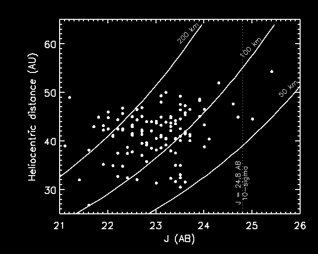
Fig. 1 - Apparent magnitudes for Kuiper Belt objects of 50, 100 and 200 km radii, assuming a 4% albedo compared to the APOGEE survey limit. APOGEE can find a 70 km object at 48 AU, the location of the Neptune 2:1 mean motion resonance. The points represent the population of KBOs with well determined orbits from the Minor Planet Center. The 10-sigma limit of the APOGEE survey represents a significant increase in depth. The observed V magnitude is transformed to J by adopting V-J(AB) = 1.0 mag (Davies et al. 2000).Ecliptic Longitude Completeness: The first year APOGEE survey of KBOs will be unprecedentedly complete in its coverage of ecliptic longitude. Longitude variations in the sky density of KBOs should become visible for the first time as resonant objects come into perihelia at preferred angular displacements from Neptune. These variations enable a statistical census of resonant membership and a test of the theory of resonance sweeping by Neptune. The reported asymmetry in the longitude distribution of objects in the 3:2 resonance (Millis et al. 2001)---which, if real, implicates Pluto as a significant perturber within this resonance (Yu & Tremaine 1999)---can be verified.
Planet X: The APOGEE census of the outer Solar System will constitute the most thorough search yet for ``Planet X''. M. E. Brown's unpublished ecliptic survey (+/-9 deg.) using the Palomar 48-inch telescope surpasses Tombaugh's pioneering search but was still confined to 120 degrees of longitude and V ~ 19-20 mag. Current limits on the amount of material in the outer Solar System, based on the absence of observable perturbations to the orbits of short-period comets, require less than 1.3 Earth masses at 50 AU (Hamid, Marsden, & Whipple 1968). Larger masses can reside at greater distances. An Earth-sized planet with KBO-like albedo (4%) at 450 AU gives a 10-sigma detection, and moves 0.5 arc sec. in 2 hours or 2 arc min. in a year.
Orbital Inclinations: Each KBO discovered during the first year of observations will have their positions measured twice over a time interval of 2 hours with astrometric precision of < 0.02 arc sec. The two orbital parameters most accurately determined from a 2-hour arc will be the inclination and the heliocentric distance . Fig. 2 demonstrates that resulting uncertainties in the inclinations are typically 0.7 degrees---an order-of-magnitude improvement over what can be done from the ground over a similar time baseline. This uncertainty is small compared to characteristic widths of KBO inclination distributions, estimated roughly to be 30 degrees. A sample of 3400 inclinations would permit a direct and definitive test of the prediction that the inclination distribution of KBOs be identical to that of short-period comets (Duncan, Quinn, & Tremaine 1988), free of the small number KBO statistics (Millis et al. 2001) and model-dependent caveats (Brown 2001) that plague current tests.
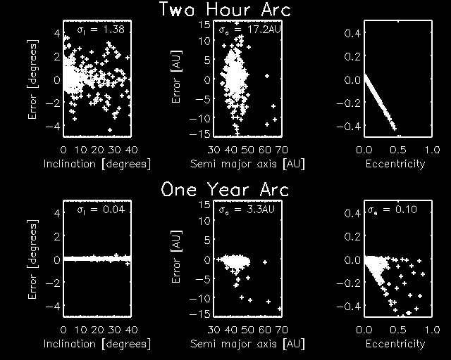
Fig. 2 - Results of simulated orbit determination from APOGEE survey data with two hour and one year arcs. The x-axis is the true value of the orbital element and the error plotted on the y-axis is the difference between the recovered and true value. Orbital elements and magnitudes are drawn from the currently known distribution of KBO's. In the four hour arc the instantaneous heliocentric distance and the inclination are well constrained. The orbit is determined with sufficient precision to recover the objects in the following year (Fig. 3). The one year arc yields determination of all six orbital elements.
The Edge of the Solar System: First epoch APOGEE measurements
yield uncertainties in their heliocentric distance of < 2 AU. A snapshot
of the instantaneous heliocentric distance distribution of 3400 KBOs would
test the controversial observation that the classical Kuiper Belt appears
to truncate at 47 AU (Jewitt, Luu, & Trujillo 1998; Gladman et al.
2000; Chiang & Brown 1999; Allen et al. 2001; Trujillo &
Brown 2001). Whether there exists an edge to the Solar System has implications
for the planet formation process and for the possibility of a stellar encounter
in the Solar System's early history (Ida et al. 2000). As Fig. 1 demonstrates,
APOGEE can easily detect 200 km diameter objects at < 55 AU.
Follow-Up Ground-Based Observations: The brightest KBOs identified by APOGEE can be observed from the ground to determine their (1) surface reflectance spectra, and (2) possible multiplicity. Fewer than ten currently known KBOs are bright enough to have their near-IR spectra measured by Keck (Brown, Blake, & Kessler 2000; Brown 2000); APOGEE would increase this target list to ~ 110. The masses of binary KBOs can be determined if they can be resolved by adaptive optics systems (Veillet 2001).
Follow-Up Space-Based Observations: Armed with precise orbital elements from the APOGEE catalog of bright Kuiper Belt Objects, SIRTF (assuming a 5 year lifetime) and NGST (launch 2009) will measure the far infrared emission of KBOs. Combining reflected and emitted fluxes yields albedos and sizes. Presently only 3 KBOs have had their sizes measured by this technique: Pluto, Charon, and Varuna (Jewitt, Aussel, & Evans 2001). Combining size and mass information in binary KBO systems yields densities---which, in turn, whether KBOs are typically cohesive bodies or agglomerations of particles bound only by self-gravity (``rubble piles'').
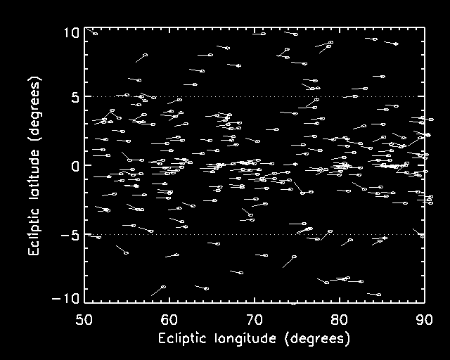
Fig. 3 - KBO's can be recovered one year later using first epoch orbital elements. This figure represents 40 degrees of longitude of the APOGEE survey; only objects with R < 24 mag are plotted. Vectors reprsent the annual KBO motion. The ellipse at the head of the vector indicates the 1-sigma uncertainties in the predicted position. In only a few cases is there any ambiguity regarding paring first epoch objects with second epoch recoveries. The surface density of objects, orbital elements and magnitudes are drawn from the currently known distribution of KBO's as in Fig. 2. The dotted horizonal lines indicate the extent of the APOGEE survey in ecliptic latitude. In one year two KBO's are lost from the survey area and three enter.Mineralogical Families: Correlations between JHK colors and orbital parameters can be investigated for the first time; currently the sample of KBOs having well-determined orbits and spectral properties is too small to permit any meaningful studies (Jewitt & Luu 1998; Brown 2000). Near-IR colors are likely to be correlated with semi-major axes in analogous fashion to the way asteroids segregate themselves into the iron, stony, and carbonaceous spectral classes with increasing heliocentric distance. Gradients in mineralogy reflect gradients in temperature and oxidizing properties of the solar nebula (Britt & Lebofsky 1999).
Exploring Ecliptic Latitude: Year three and beyond can be used to survey the outer Solar System at ecliptic latitudes > 10 degrees. Such observations would further refine the inclination distributions of the various families and increase the chances of finding highly inclined objects, be they scattered KBOs or Planet X. The possibility remains that the entire plane of the Kuiper Belt warps outward so that the bulk of objects reside at ecliptic latitudes out of the ecliptic (Hahn 2000).
The theory of white dwarf cooling, combined with the Galactic disk luminosity function (LF), has been used to date the disk at 8-9 Gyr and to show that it has had roughly constant star formation (Oswalt et al. 1996; Leggett et al. 1998; Knox et al. 1999). The luminosity function of the kinematically distinct halo population (Oppenheimer et al. 2001b) is rapidly rising toward lower luminosity, suggesting that many cooler white dwarfs may exist in the solar neighborhood that are too faint to be revealed by the existing surveys (Hansen 2001). APOGEE is designed to discover cool, dim and ancient halo white dwarfs. If the halo formed in a burst of short duration before the disk (Eggen, Lynden-Bell, & Sandage 1962), it would be possible to measure the time elapsed between the formation of both structures (Mochkovitch et al. 1990) by comparing the disk and halo white dwarf luminosity functions. If mergers of protogalactic fragments played an important role in the formation of the Galactic halo (Searle & Zinn 1978), then these events will be encoded in the white dwarf luminosity function.
Cool white dwarfs have also attracted attention because they may dominate the baryonic mass of the Galactic halo. Microlensing events toward the Large Magellanic Cloud may be produced by massive compact halo objects (MACHOs; Alcock et al. 2000); the contribution of such objects to the total halo mass is 8-35% (95% confidence) according to the microlensing experiments and at least 1% of the halo mass is in white dwarfs based on direct detection techniques (Oppenheimer et al. 2001b). White dwarfs are natural MACHO candidates because the mass distribution of lenses is similar to that of known white dwarfs. These results are contentious in part because such a large density of halo white dwarfs is inconsistent with the current field IMF: Using the known population of halo main-sequence dwarf and a Salpeter IMF, Gould et al. (1998) estimated that halo white dwarfs could account for no more than 0.2% of the halo mass.
Additional data related to this problem has arisen recently because unambiguous halo white dwarfs have been identified, e.g., WD 0346+246 (Hambly et al. 1997, Hodgkin et al. 2000, Oppenheimer et al. 2001a), and F351-50 (Ibata et al. 2000). Oppenheimer et al. (2001b) have reported a detection of the bright tail of the halo white dwarf population. These results, along with independent statistical analysis (e.g. Koopmans and Blandford 2001) and survey work (Monet et al. 2000, Liebert 2001) imply that the halo white dwarf population is at least 8 times larger than Gould et al.'s (1998) limit. The characterization of the halo white dwarf luminosity function is of paramount importance to the nature of star formation itself because these new observations seem to require evolution of the IMF.
The number of known cool white dwarfs is small, with a few objects per
luminosity bin in both the disk and the halo. Since the coolest white dwarfs
carry the most weight in determining the age and formation history, sampling
statistics alone yield age errors for the disk of about 1 Gyr, comparable
to the systematics in the evolutionary models. Fontaine et al. (2001)
show that recent advances in interior and atmospheric physics for white
dwarfs will reduce these errors such that the observational sampling errors
will dominate. An order of magnitude increase in the sample size of cool
white dwarfs is thus necessary and timely, enabling determination of ages
to within a few percent (Knox et al. 1999), a reliable measurement of the
halo white dwarf mass density and hence measurement of the primordial IMF.
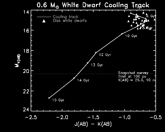
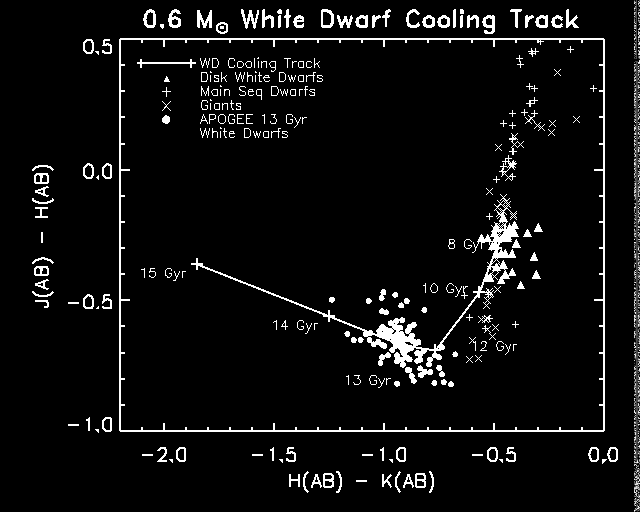
Figure X. Selection technique and rough volume estimate for the APOGEE survey for cool white dwarfs. The solid line in both (a) and (b) shows a cooling track for a 0.6 solar mass white dwarf (Chabrier et al. 2000) and illustrates the extreme infrared colors predicted for an ancient (> 10 Gyr) white dwarf. (a, left): The near-IR color-color diagram for white dwarfs.. The filled circles show a hypothetical 13 Gyr old halo white dwarf population detected in a simulated 900 sq. degree APOGEE survey (see text for details). 121 white dwarfs were found within 230 pc (median 175 pc). Collisionally induced H2 absorption in cool (< 4000 K) white dwarf atmospheres distinguishes them from all other known celestial objects. The Leggett et al. (1998) disk sample of white dwarfs is plotted along with other stellar types for reference. LHS3250 and WD0346+246, two well-studied white dwarfs with CIA, are marked with open squares to show that the predicted colors are realistic. (b, right): Absolute K(AB) magnitude and J-K color used to estimate the depth of the snapshot survey. The triangles are the same as in (a) for the Leggett et al. white dwarfs with a mean distance of 15 pc. For white dwarfs with an age equal to13 Gyr, the APOGEE snapshot survey explores10 times more volume than already sampled. A more detailed simulation of the volume of the survey (partial results in (a)) is explained in the text.The APOGEE assembly of a vastly expanded sample of cool white dwarfs is significant in its own right because of the physics accessible through follow-up studies to determine temperatures, ages and atmospheric compositions. However, the only way to separate the kinematically distinct halo and disk populations is by inferring the kinematics of each star by measuring proper motions; radial velocities cannot be measured for cool white dwarfs because the spectra lack any fine features. Strictly speaking proper motion can only be converted into physical velocity if the distance is known, but because the radius of a white dwarf changes insignificantly with age and weakly with mass, the use of a color-magnitude relation results in distance determinations with an accuracy of about 20%, sufficient for distinguishing halo and disk populations (Oppenheimer et al. 2001b). The APOGEE snapshot survey will find objects like the faintest known white dwarf, WD0346+246 (MK = 16.8), out to 525 pc. Any candidate within this distance with typical halo velocities (< vphi> ~ -185 km/s ) will have a proper motion of >~ 70 mas/yr. For a point source detected at 10-sigma significance, the astrometric accuracy will be approximately 15 mas (0.1 pixel). Thus halo kinematics can be detected at 5-sigma significance for stars as distant as 525 pc. The astrometric reference frame will be provided by a minimum of 3300 galaxies and 55 stars (K < 25.3 AB) per chip in the highest Galactic latitude fields.
For an object like WD 0346+246 Oppenheimer et al.'s (2001b) proper motion survey probed about 7x10⁵ pc3 and found about 20 candidate halo white dwarfs. If this white dwarf is a prototypical halo member, then a rough estimate of the volume of the APOGEE survey is 1.4x10⁷ pc3 after one year at a nominal rate of 2.5 sq degrees/day. Clearly, the order of magnitude sought in the statistics of the LF is feasible.
Predicted Number Densities
We have conducted a more detailed simulation to refine the estimate of the survey volume and number of cool white dwarfs APOGEE will discover. Isern et al. (1998) have calculated theoretical luminosity functions of halo white dwarfs assuming that the halo forms in a burst of duration 0.1 Gyr and has a Salpeter initial mass function (IMF). We normalize that luminosity function to the data of Leibert et al. (1988; 1989) at MV = +13.5). This is a conservative assumption, since it corresponds to a space density which represents at most 0.6% of the local dark halo density of 0.01 solar masses per cubic parsec (Gilmore 1997), similar also to the Gould et al. (1998) estimate---the results of the Oppenheimer et al. (2000b) proper motion survey and the new analysis of the Liebert sample (Monet et al. 2000, Liebert 2001) imply space densities several times larger, requiring biassed IMFs, which favor the formation of white dwarfs (Adams & Laughlin 1996; Chabrier, Ségretain and Méra 1996).
The number of detectable halo white dwarfs declines with the cooling
age of the population. To be conservative yet realistic, we take the maximum
age by assuming that the halo is as old as the oldest globular clusters.
Recent estimates give 11.5±1.3 Gyr; including Hipparcos-based statistical
parallax measures for halo sub-dwarfs, raises the mean age to 12.8±1Gyr
(Krauss 2000). On this basis we expect about 900 halo white dwarfs
per steradian in the APOGEE survey at J < 25.2 AB, 10-sigma. Table
X shows the calculation for a variety of ages and assumed IMFs.
|
|
|
|
|
|
|
|
|
|
|
|
|
|
|
|
|
|
|
|
|
|
|
|
|
|
|
|
|
|
These calculations show that the survey area required to expand the number of known halo white dwarfs by a factor of 10 is 900 square degrees. We have performed numerical experiments adopting a halo that formed in an instantaneous burst 13 Gyr ago with a Salpeter IMF and a halo white dwarf mass density of 0.6% of the local dark halo density. The 900 square degree survey yields about 120 white dwarfs (J < 25.2 AB, H < 25.2 AB, 10-sigma & K < 26.0 AB 5-sigma). We have plotted the results of one such experiment on the J-H/H-K color-color diagram (Fig. X(a)) to show that these cool white dwarfs are cleanly separated from their younger disk siblings and Galactic stars. The formal uncertainty in the age of the population, as derived from the spread in the H-K color, is 0.2 Gyr 1-sigma, indicating that we have sufficient precision not only to date the halo, but to reconstruct the halo star formation history for the first time. Many cool disk white dwarfs will also be found. These can be used to improve the disk age derived from the disk LF. It is important to note that this is conservative. If the Oppenheimer et al. (2001b) result is correct, if the halo is younger than the globular clusters, or if the microlensing detections are halo white dwarfs, the numbers of halo dwarfs will vastly exceed this estimate. For example, the ad hoc initial mass functions of Adams & Laughlin (1996) and Chabrier, Ségretain, & Méra (1996), which explain the MACHO microlensing events in terms of halo white dwarfs, predict an order of magnitude more objects and 4-10% of the dark halo for any reasonable age of the Galaxy.Numbers in parenthesis for the Salpeter IMF are the numbers of white dwarfs detected by the SDSS in r'-band at < 22.3 AB, 10-sigma. Note: it is impossible to identify these objects as white dwarfs on the basis of SDSS data alone. APOGEE is the only survey that can identify them as white dwarfs uniquely. AL & CSM are biassed IMFs (Adams & Laughlin 1996; Chabrier,
Ségretain & Méra 1996) which favor white dwarfs.
In any case, the principal requirements of a survey needed to solve
the white dwarf problem are the ~107 pc3 survey volume for obects
like WD 0346+246 and 5-sigma proper motion detections. Apogee stands
alone as the only survey capable of this. The Hubble Deep Field
is so narrow that it cannot constrain the numbers of halo white dwarfs
(Isern et al 1998). Pencil-beam surveys have no chance at solving
this problem, even if their depth goes to the edge of the Galactic halo.
No ongoing or proposed space mission, e.g., SIRTF, PRIME, NGSS, FAME, SIM,
GAIA, or NGST, combines the necessary depth, area and astrometric accuracy.
The Sloan Digital Sky Survey (SDSS) cannot discover cool white dwarfs because
the usable colors are not capable of uniquely identifying white dwarfs,
and there will be no proper motions except within some very limited strips
on the sky. Thus, halo white dwarfs will go unnoticed. The
potential competition from the ground may be the proposed Large-aperture
Synoptic Survey Telescope (LSST) or the UK's Visible and Infrared Survey
Telescope for Astronomy (VISTA), both of which will begin collecting data
after APOGEE's first year of observations.
Multi-color, wide area infrared sky coverage, with high sensitivity
and angular resolution are necessary to detect and identify the most distant
quasars. No other current or planned ground- or space-based mission can
find and identify these objects. These quasars are rare, and the NGST does
not have the field of view necessary to search for them.
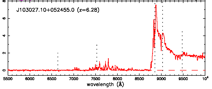
The detection of the Gunn-Peterson effect in the most distant (z = 6.28) Sloan Survey quasar (Becker et al. 2001). The implication is at higher redshifts the universe is opaque to rest frame emission at wavelengths < 1216 A, and z > 7 quasars will only be detectable at wavelengths longer than 1 micron. The Ly-alpha absorption in high redshift quasars evolves strongly with redshift. For z < 5.7, the Ly-alpha absorption is as expected from lower redshifts, but in this, the highest redshift object, the flux 8500-8700 A is consistent with zero. The flux level drops by a factor of > 150, and is consistent with zero in the Ly-alpha forest. This is a clear detection of a complete Gunn-Peterson trough, caused by intergalactic HI. The fast evolution of the absorption in high-z quasars suggests that the ionizing background has declined significantly from z = 5- 6, and the universe is approaching the reionization epoch at z ~ 6.Recent results from the Sloan Digital Sky Survey show that the most distant quasars (z ~ 6) are probing the threshold of the hydrogen reionization epoch (Becker et al. 2001). For z = 7 the Gunn-Peterson absorption of intergalactic HI will extend to 0.97 microns, indicating that infrared observations are necessary to find the most distant quasars and to probe the sequence of events that occur during the epoch of reionization. Extrapolation of the 3.5 < z < 5.0 quasar luminosity function suggests that over 1000 quasars with 6 < z < 10 can be detected by APOGEE.
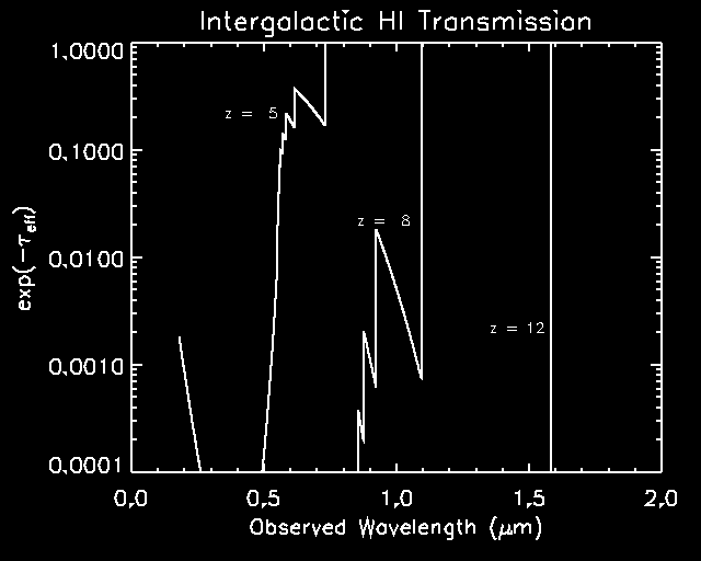
A high redshift analog of the exceptionally luminous 3C273 (MB = -26.8) at z = 8 has K = 20.5 AB. Taking MB < -23 as the definition of the boundary between lower luminosity AGN and quasars, the APOGEE snapshot survey has sufficient sensitivity to find all quasars to z = 14!Average transmission of the universe as a function of the observed wavelength for emission redshifts z = 5, 8 and 12 (Madau, 1995). The characteristic staircase profile is due to continuum blanketing from the HI Lyman series. By z = 8 the opacity of the intergalactic medium effectively extinguishes rest frame emission at wavelength shorter than 1216 A, corresponding to an observed wavelength of 1 micron. At high redshifts, only infrared observations are practical because the universe is opaque to shorter wavelength radiation. Infrared observations are favored even more strongly than suggested by this plot because the intergalactic opacity adopted here does not include the onset of increased absorption at z > 5.5 associated with the formation of a complete Gunn-Peterson trough (Becker et al. 2001).
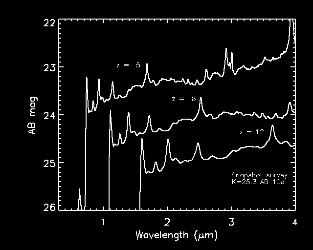
Fig. X - Predicted fluxes for low luminosity (MB = -23) high redshift quasars (H0=50 km/s/Mpc, Omega=0.3, Lambda = 0.7) based on the composite spectrum of Vanden Berk (2001). Taking MB < -23 as the operational definition of a quasar APOGEE can detect all quasars with z < 14. High redshift quasars, e.g., z=8 are undetectable shortward of 1 micron; the drastic decline in flux shortward of 1216 A in the rest frame is due to intergalactic HI absorption. An exceptionally luminous quasar such as 3C273 is 3.8 mag brighter.While quasars as luminous as 3C273 are likely to be rare at high redshift because of the steepness of the luminosity function with absolute magnitude and limited volume at high redshift interval extrapolation of the SDSS luminosity function measured for the redshift range of 3.6 < z < 5.0 (Fan et al. 2001) suggests that more typical quasars are plentiful. If this extrapolation is valid then there are ~ 1020 quasars 6 < z < 10 within the nominal area of sky (3600 square degrees) accessible to APOGEE. Theoretical estimates of the abundance of quasars tend to be more optimistic by factors of two to three than formal extrapolation of the quasar luminosity function. The table compares the extrapolation of the SDSS luminosity function with the predictions of Haiman & Loeb (1998) for a Lambda-CDM cosmology in which an early population of quasars (MB < -23) reionizes the universe.
|
|
|
|
|
|
|
|
|
|
|
|
|
|
|
|
|
|
|
redshift/str * |
|||||||
|
|
|
|
|
|
|
|
|
|
|
|
|
|
|
|
|
|
* Extrapolation of the SDSS 3.6 < z < 5 quasar luminosity function (Fan et al. 2001).
** Theoretical quasar luminosity of Haiman & Loeb (1998) normalized at z=5.
Based on these numbers, we need to survey between 300-900 square
degrees to have a 95% probability of finding ten or more z = 8 quasars.
There is also a 99% chance that the first year will net one z = 9 quasar.
By the third year of the mission we expect to have covered 1800 sq degree
and found between 30-100 z = 8 quasars. With this number of quasars it
will be feasible to make quantitative studies of the luminosity function,
and decide, for example, whether or not quasars are responsible for reionization.
Extrapolations of the quasar luminosity function is highly uncertain. However, there are theoretical reasons to expect that high redshift quasars will be be detected in deep infrared surveys. Dynamical studies indicate that remnant black holes indeed in the quiescent nuclei of most nearby galaxies (Magorrian et al. 1998; Ferrarese & Merritt 2000; Gebhardt et al. 2000), and imply that black hole formation is a generic consequence of galaxy formation. The recent discoveries of luminous quasars at z ~ 6 imply that black holes more massive than a few billion solar masses were already assembled when the universe was less than a billion years old. The presence of these black holes is not surprising in popular hierarchical models of structure formation. For example, the black hole needed to power the quasar SDSS 1044-0125 at z = 5.8 could arise naturally from the growth of stellar-mass seeds forming at z ~ 15, when typical values are assumed for the radiative accretion efficiency and the bolometric accretion luminosity in Eddington units.
Haiman & Loeb (2001) combine constraints of high redshift
Sloan quasars with a simple model for appearance of the first quasars by
parameterizing the growth of seed black holes in terms of radiative accretion
efficiency, the bolometric accretion luminosity in Eddington units,
the minimum halo velocity dispersion, and the seed mass. The first
step is to determine the mass of the halo in which a quasar of luminosity,
L, resides by equating the observed number of quasars brighter than L to
f(z)N(M, z), where N is the integral number of halos with mass >
M per unit solid angle, per unit redshift and f(z) is the fraction of halos
hosting active quasars. Here N is estimated using the extended Press-Schechter
formalism. Because of the exponential shape of the halo mass function for
rare halos, the inferred halo mass depends only logarithmically on f(z)
and f(z) ~ 1 is a conservative assumption. The growth of the central black
hole depends on the assembly of its host halo. Given a halo of total mass
at a redshift z, the EPS formalism specifies its average merger history
at higher redshifts. The mass of each seed black hole is assumed
to grow exponentially by accretion from the formation time of the seed.
Eventually all massive black holes merge together to form a single supermassive
black hole at the center of the parent halo.
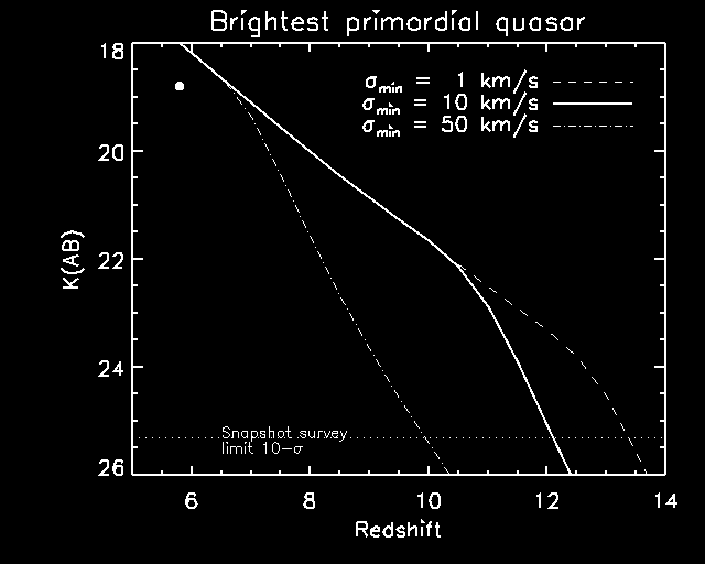
Fig. X - The brightest quasar found in a 10 square degree survey per unit redshift interval is plotted versus redshift (Haiman & Loeb 2001). The solid curve corresponds to a black hole seed mass of 10 M(sun) and a minimum velocity dispersion of 10 km/s appropriate for HI cooling of gas with primordial abundances. The radiative accretion efficiency is 0.06 and the bolometric accretion luminosity in Eddington units is 1. The black hole is conservatively only allowed to consume 1% of the available gas in its host halo. The high value of the the velocity dispersion applies if the limiting mass for a progenitor halo is determined by feedback from the UV background following the reionization epoch and the low value applies before reionization if sufficient H2 exists to allow cooling in small halos. The filled circle shows the z = 5.8 quasar SDSS 1044-0125.
The results of these calculations suggest that it is likely that
the APOGEE survey will probe the first generation of quasars at z > 10.
For standard assumptions the APOGEE snapshot survey penetrates to z ~ 12.
High redshift quasars are predicted to be abundant; there are about 300
per unit redshift interval per steradian. Except for the lowest redshift
examples, z ~ 6, these primordial quasars are more abundant than extrapolation
of the 3.6 < z < 5 SDSS quasar luminosity function. Under the
most pessimistic condition when the black hole is allowed to consume only
1% of the gas in its host halo, and the velocity dispersion is enhanced
by feedback from the UV background the APOGEE survey penetrates to z ~
10.
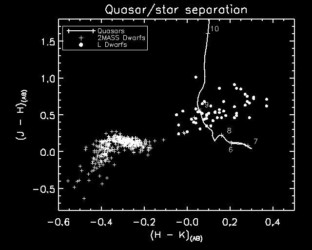
Fig. X - The colors of quasars (solid line labeled with redshifts) change gradually between z = 5 and 8 and then redden dramatically in J-H as Ly alpha is redshifted out of the J band at z = 9.5. High redshift quasars (6 < z < 8) are cleanly separated from Galactic stars in the J-H, H-K color color diagram. The major contaminant for z ~ 9 quasars are mid-L dwarfs, but these quasars will be identified as i'- and z'-band drop outs. The 2MASS dwarfs are stars within 25 pc from the NSTARS database. The L-dwarfs are from Kirkpatrick et al. (1999; 2000)
In the future, integral field spectrometers that implement OH avoidance,
and are fed by a laser guide-star adaptive optics system will offer a 1.5-2
mag advantage. Thus advances in adaptive optics will make an order of magnitude
more targets observable from the ground. Ultimate spectroscopic exploitation
of the APOGEE quasars requires NGST. A typical quasar (MB
= -23) at z = 9 will require a13 hour exposure for the same resolution
and SNR.
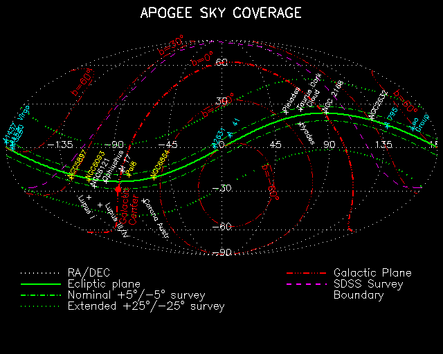
Fig. 1 - Sky coverage shown in celestial coordinates. APOGEE can point continuously in the anti-solar direction within a nominal survey band of +/- 5 degrees of the ecliptic (dot-dash green), corresponding to approximately 9% of the sky. The spacecraft surveys Galactic latitudes of -63o < b < +63o. This zone includes a broad variety of potential targets: solar system, Galactic, and extra-galactic, including local dark clouds and star forming regions (e.g., Ophiucius, Taurus), open clusters (e.g., Pleiades), globular clusters (for clarity only a few are plotted), the Galactic Center and clusters of galaxies (e.g., Virgo, Abell 41 at z=0.28). 36% of the nominal APOGEE survey band is covered by the Sloan Digital Sky survey. The purple line shows the southern limit of the SDSS's north Galactic cap survey. The dot-dash green lines show the region of sky that can be observed without repointing the telescope when it crosses the equator. The extended zone is accessible if the space craft is repointed twice per orbit. The green dotted lines show the ecliptic latitudes accessible when the space craft is north (south) of the equator are -5o < b < +25o ( -25o < b < +5o).
The limiting natural background in low earth orbit is zodiacal light. Interplanetary dust scatters sunlight and emits thermal radiation. The best measurements of this background at these wavelengths have been made by the DIRBE experiement on COBE. The contour plots show the distribution of zodiacal light at 2.2 microns derived from Kelsall et al.'s (1998 ApJ, 504, 44) COBE/DIRBE zodiacal light model. APOGEE is constrained to point at the anti-solar direction: lambda = 0 degrees on September 21, lambda = 90 degrees on December 21, lambda = 180 degrees on March 21, and lambda = -90 degrees on June 21.
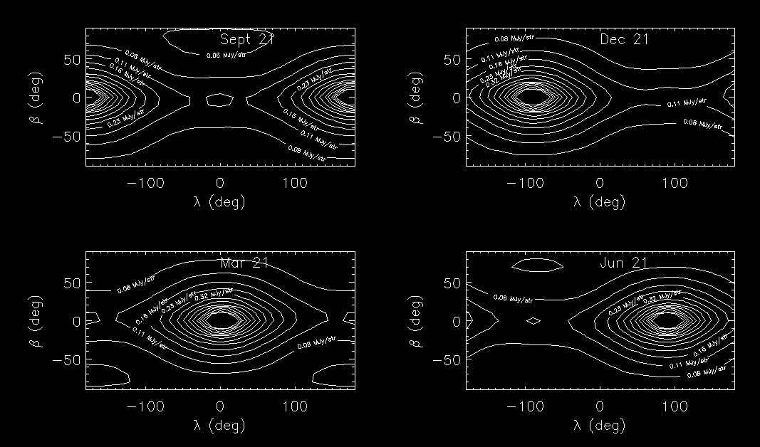
Fig. 2 - Zodiacal emission at 2.2 microns from the Kelsall et al. model of COBE/DIRBE data. Contours are labelled in MJy/sr. Peak emission is centered on the sun. APOGEE observes in the anti-sun direction, e.g., 0 degrees longitude on Sept 21. Due to back scattering, there is a minor local maximum in this direction which incurs a penalty in sensitivity compared to the ecliptic pole. However, the sun shield for a space craft which views the ecliptic plane is significantly smaller than for one which views the pole.
| Band | Wavelength
(microns) |
I (MJy/str)
Sept 21 |
I (MJy/str)
Dec 21 |
I (MJy/str)
Mar 21 |
I (MJy/str)
Jun 21 |
I (MJy/str)
Ground |
| J | 1.25 | 0.21 | 0.22 | 0.21 | 0.204 | 30 |
| K | 2.2 | 0.12 | 0.13 | 0.12 | 0.12 | 92 |
| L | 3.5 | 0.054 | 0.058 | 0.054 | 0.052 | 1.29e+05 |
| M | 4.9 | 0.22 | 0.25 | 0.22 | 0.205 | 1.30e+07 |
At short wavelengths (J & K), back-scattered light in the anti-solar direction incurs a penalty in background of approximately x 2 compared to a telescope that views the ecliptic pole. For comparison, the sky brightness for Mauna Kea (Shure et al. 1994 ) is tabulated.
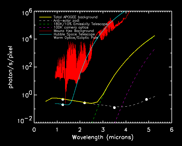
Fig. 3 - The APOGEE background (yellow) is dominated by zodiacal light at wavelengths less than 2.8 microns. Filter bandwidths of 20% are adopted. At longer wavelengths thermal emission from the cool (180 K) telescope optics dominate. The filled white dots are the Kelsall et al. DIRBE points approriate for APOGEE and HST. The APOGEE background is about three orders of magnitude less than the ground over most of the operating wavelength range. The HST (cyan) and ground-based (red) backgrounds are comparable beyond 2.0 microns because the Hubble optics are warm. Hubble has a slight advantage at wavelengths less than 1.6 microns because it can view the ecliptic pole where scattered zodiacal light is a minimum.
| Subsystem | Parameter |
|
| Telescope | ||
| Collecting area |
|
|
| Throughput |
|
|
| Emissivity |
|
|
| Temperature |
|
|
| WFE |
|
|
| Camera | ||
| Throughput |
|
|
| Temperature |
|
|
| Pixel size |
|
|
| Detector | ||
| Read noise |
|
|
|
|
||
| Dark current |
|
Read noise is quoted for Correlated double sampling (CDS) and multiple correlated double sampling (MCDS)
|
|
|
|
|
|
|
|
|
SNR |
|
|
|
|
|
|
||||
|
|
|
|
|
|
|
|
|
8.1 |
|
|
|
|
|
|
|
|
|
9.2 |
|
|
|
|
|
|
|
|
|
0.9 |
|
|
|
|
|
|
|
|
|
0.04 |
Exposure time = 200 s, filter bandwidth = 25%.
Assumes two cosmic-ray split 100 s exposures. Detector noise lists the combined variance of dark current and read noise. For Poisson statistics the variance equals the mean and so the magnitude of noise sources can be compared.Thermal emission from the interior of the camera dewar at 100 K is an order of magnitude lower than thermal emission from the telescope optics.
N(pix) is the number of pixels in the detection aperture. Photometery is performed in an aperture which encircles 80% of the light, or 4 pixels, which ever is larger.
The L & M bands are shown for comparison only. The APOGEE focal plane will not include detectors which operate at this wavelength.
|
|
|
|
|
|
|
|
|
|
|
|
|
|
|
|
|
|
|
|
|
|
|
|
|
|
|
|
|
|
|
|
|
|
|
|
For each detector array sixteen million pixels per array are read out over 32 parallel channels with 5 microscond conversion. Sixteen reads per pixel are used so that that the total readout time is 10.4 seconds. The array is read non-destructively during the exposure to veto cosmic rays (Stockman et al. 1998) so there is only 660 ms of overhead per exposure. The 5' telescope slew takes 7 seconds (0.3 Nm reaction wheel and I = 2500 km m2) and the fine guidance system takes 30 seconds to acquire the new field and stablize the scene to 0.03 arc sec. rms. The total time available in survey mode for science exposures is 400 s per field, i.e., 2 x 200 s. We cover 2.5 sq degrees per day, or ~ 900 sq degrees per year. In the second year we re-visit one half of the fields so that we have accumulated one epoch for 1350 sq degrees and two epochs, for proper motions, for 450 sq degrees. In the third year we repeat this strategy so that at the end of the nominal mission we have observed 1800 sq. degrees with at least one epoch and 900 sq. degress with two epochs.25 AB = 360 nJy. The conversion between the Vega and AB system is J - J(AB) = -0.91, H-H(AB) = -1.38, K-K(AB) = -1.89, L-L(AB) = -2.78, & M-M(AB) = -3.43Survey mode consists of two co-added 200 s exposures separated by 4 hours.
The exposure time for one orbit is for an elapsed time of 6200 s (one orbit) and 80% observing efficiency. Ultra deep corresponds to 120 orbits or 10 days elapsed time with 80% efficiency. This is the maximum exposure time given by the nominal +/- 5 degree pointing constraints.
The nominal APOGEE survey spans -63 to +63 degrees in Galactic latitude: the average height above the galactic plane over the course of a year is 36 degrees. In an ultra-deep survey (K = 29.5 AB, SNR=10) and the median integrated star count is 37,000 per square degree or 10 stars per square arc minute. At low Galactic latitude source confusion noise, and not photon fluctuations, will set the limiting magnitude. Before this regime is approached photometry becomes unreliable. Our requirement for systematic errors in photmetry is < 2%, which simulations using SKY show is met if there are 50-100 pixels per star. Suppose we do aperture photometry in an aperture which encircles 80% of the stellar light. This criterion is equivalent to requiring that a 3x3 swatch of apertures contains one star. At K band this corresponds to one star per 90 pixels or 1 per square arc second (1.3e+07 stars per square degree).
The APOGEE line of site crosses the Galactic plane at the center and
anti center directions where star counts peak at 1.3e+06 and 1.9e+08 stars
per sq. degree respectively in the deepest fields. A few percent (<4%)
of the survey field are dominated by source confusion noise. The
minimum star count is 8040 stars per square degree or 55 stars per 2048
x 2048 quadrant of the focal plane. The brightest star per quadrant at
highest latitudes will be K < 15 AB, which yields a peak count 410,000
photoelectrons in the brightest pixel or a total of 1.3e+04 photoelectrons
per second. This will cause saturation, but hybrid focal plane arrays do
not suffer from bleeding which is common in CCD. The bright stars will
be suitable for correcting residual tip-tilt errors.
| K < 25.3 AB | K < 26.8 AB | K < 29.5 AB | |
| Minimum | 8040 | 9590 | 11,100 |
| Median | 26,000 | 31,300 | 37,600 |
| Max (anticenter) | 9.56e+05 | 1.22e+06 | 1.31e+06 |
| Max (center) | 5.67e+07 | 9.46e+07 | 1.89e+08 |
| Percentage of confused
survey fields |
3.0% | 3.3% | 3.6% |
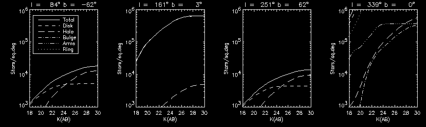
Fig. 4 - Cumulative K-band star counts for four equi-spaced epochs during the APOGEE survey. The median galactic latitude of the survey is 36 Typical star densities correspond 30,000 stars per square degree or 10 stars per square arc minute. to In the anticenter direction APOGEE star counts are dominated by the disk. At high latitude the contribution of disk stars has converged by K = 24.3 AB Beyond this point halo stars dominate and their counts converge by K = 27.3 AB.
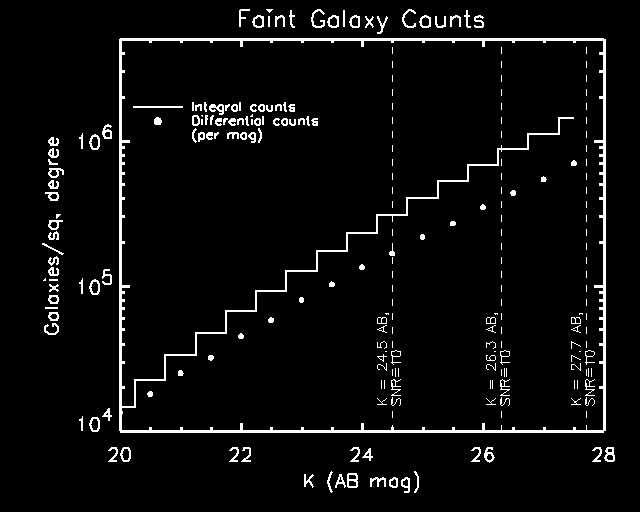
Merged faint galaxy counts from Yan et al. (1998) for H < 25.9 AB, Bershady et al (1998) for K < 24.9 AB, Thompson et al (1999) for H < 28.8 AB. The data have been corrected for incompletness according to Thompson et al. Beyond K = 27.5 AB there are significant uncertainties due to small field observed by NICMOS, photometric errors, and statistical errors. The SNR = 10 thresholds for snap-shot, deep, and ultra deep APOGEE surveys are shown.The figure shows that the APOGEE snapshot survey will collect near IR photometric and structural information for approximately 300 million faint galaxies. Galaxies do not present a significant source of confusion in the snapshot (4.7e5 galaxies/sq. degree) or deep (1.0e6 galaxies/sq. degree) survey modes. In the ultradeep mode galaxy counts are uncertain, but galaxies probably still cover < 1% of the sky. The approximately 3000 galaxies K < 25.3 AB per chip (5' x 5') in the snapshot survey will provide the reference frame for relative astrometry to meausure proper motions of stars and to identify moving solar system objects. Systematic effects due to errors in the detector lithography masks, optical distortions, undersampling in J and H, and the irregularity of galaxies limit our precision to 1-3 mas.
The principal invesigator is Dr. James R. Graham, a professor
of Astronomy at the University of California Berkeley. He has built
infrared instruments for Lick (the AO camera IRCAL) and Keck Observatories
(project scientist of NIRSPEC), and and led the Imaging Fourier Transform
Spectrometer study for NGST. Dr Graham will be responsible for the integrity
of the proposed scientific investigation, and all phase of the mission
development, including instrument design, science verification, observing
program planning, and operations, eduction and outreach, and the archiving,
analysis, distribution, and publicationof APOGEE data.
Dr Eugene Chiang is a professor of Astronomy and Earth & Planetary Sciences at the UC, Berkeley specializing in dynamics. His relevant expertise includes the Kuiper Belt, which he will use to define the APOGEE solar system science.
Dr Ray Jayawardhana is a professor of Physics at the University of Michigan. His area of expertise is the formation of stars and planets. His repsonsibilities include the starformation science with APOGEE.
Dr Paul Kalas is reseach astronomer at UC Berkeley, who will contribute to the science team his knowlege of instrument design, zodiacal dust clouds (solar and extra-solar) and extensive knowlege of space astronomy.
Dr Michael Lampton is a senior Fellow at Space Science Lab, UC, Berkeley. He has 30 years building and testing spaceborne telescopes, and for APOGEE his skills and experience will be utilized in the development, procurement, and test of the proposed optical system.
Dr Ben Oppenheimer is a Hubble Fellow at the American Museum of Natural History where he will lead the activities related to cool white dwarfs. He brings his experise in astronomical instrument design, astrometry, and the physics of cool white dwarfs. Dr Oppenheimer will also lead the AMNH's contributions to the EPO program.
Dr. Schuyler VanDyk, a staff scientist at IPAC, brings his very high familiarity with the construction and operations of the 2MASS processing pipeline and with its data products generation and dissemination to the astronomical community. Scientific interests in APOGEE include galaxy evolution and Galactic high-mass star formation and evolution.
Dr David Frayer
Dr Martin White is a professor of Physics and Astronomy at UC, Berkeley. He is a theoretical cosmologist, and will plan and develop the observing strategy for finding and characterizing high redshift quasars.
Alcock, C., et al. 2000, ApJ, 542, 281
Allen, R.L., Bernstein, G.M., & Malhotra, R. 2001, ApJL, 549, L241
Barkana, R., & Loeb, A. 2001, Phys Rep, 349, 125 ( astro-ph/0010468)
Becker, R. H., et al. 2001, astro-ph/0108097
Bennett, C. L., Banday, A. J., Gorski, K. M., Hinshaw, G., Jackson, P., Keegstra, P., Kogut, A., Smoot, G. F., Wilkinson, D. T., & Wright, E. L. 1996, ApJ 464, 1
Bernstein, G., & Khushalani, B. 2000, AJ, 120, 3323
Bershady, M. et al ApJ, 505, 50, 1998
Britt, D.T., & Lebofsky, L.A. 2000, in Encyclopedia of the Solar System}, ed. P. L. McFadden, & T. Johnson, 585
Brown, M.E. 2000, DPS Meeting #32, #20.08
Brown, M.E., Blake, G.A., & Kessler, J.E. 2000, ApJL, 543, L163
Brown, M.E. 2001, AJ, 121, 2804
Chabrier, G., Ségretain, L., & Méra, D. 1996, ApJ, 468, L21
Chabrier, G., Brassard, P., Fontaine, G., & Saumon, D . 2000, ApJ, 543, 216
Charlot, S., & Silk, J. 1995, ApJ, 445, 124
Cohen, M. 1994, AJ, 107, 582
Chiang, E.I., & Brown, M.E. 1999, AJ, 118, 1411
Davies, J.K., et al. 2000, Icarus, 146, 253
Duncan, M.J., & Levison, H.F. 1997, Science, 276, 1670
Duncan, M., Quinn, T., & Tremaine, S. 1988, ApJL, 328, L69
Eggen, O. J., Lynden-Bell, D., & Sandage, A. R. 1962, ApJ, 136, 748
Fan, X. 2001, AJ, 121, 54
Ferrarese, L., & Merritt, D. 2000, ApJ, 539, L9
Fryer, C. L. 1999, ApJ, 522, 413
Fontaine, G. Brassard, P., Bergeron, P. 2001, PASP, 113, 409
Gebhardt, K., et al. 2000, ApJ, 539, L13
Gil-Hutton, R.; Licandro, J. 2001, Icarus, 152, 246
Gladman, B., et al. 2000, DPS Meeting #32, #20.03
Gnedin, N. Y., & Ostriker, J. P. 1997ApJ, 486, 581
Gould, A., Flynn, C., Bahcall, J. N. 1998, ApJ, 503, 798
Haiman, Z., Thoul, A. A., & Loeb, A. 1996, ApJ, 464, 523
Haiman, Z. & Loeb, A. 1998, ApJ, 503, 505
Haiman, Z. & Loeb, A. 2001, ApJ, 552, 459
Harris, H. C., Dahn, C. C., Vrba, F. J., Henden, A. A., Liebert, J., Schmidt, G. D., & Reid, I. N. 1999, ApJ, 524, 1000
Hambly, N. C., Smartt, S. J., Hodgkin, S. T., 1997, ApJ, 489, L157
Hambly, N. C. & Oppenheimer, B. R. 2002, in "The Future of Small Telescopes," T. Oswalt, ed. (Kluwer), in press
Hansen, B. M. S. 2001, ApJ, 558, L39
Hodgkin, S. T., Oppenheimer, B. R., Hambly, N. C., Jameson, R. F., Smartt, S. J., & Steele, I. A. 2000, Nature, 403, 57
Ibata, R., Irwin, I., Bienaymé, O., Scholz, R., & Guibert, J. 2000, ApJ, 532, L41
Hahn, J.H. 2000, 31st LPSC, abstract #1797
Hamid, S.E., Marsden, B.G., & Whipple, F.L. 1968, AJ, 73, 727
Ida, S., et al. 2000, ApJ, 534, 428
Jewitt, D., Aussel, H., & Evans, A. 2001, Nature, 411, 446
Jewitt, D., & Luu, J. 1993, Nature, 362, 730
Jewitt, D., & Luu, J. 1998, ApJ, 115, 1667
Jewitt, D., Luu, J., & Trujillo, C. 1998, AJ, 115, 2125
Jewitt, D., & Luu, J. X. 2000, in Protostars and Planets IV, ed. V. Mannings, A. P. Boss, & S. S. Russell, 1201
Kelsall, T., et al. 1998, ApJ, 508, 44
Kenyon, S., & Luu, J. 1998, AJ, 115, 2136
Kenyon, S., & Luu, J. 1999, AJ, 118, 1101
Kirkpatrick, J. D. et al. 1999, ApJ 519, 802
Kirkpatrick, J. D. et al. 2000, AJ 120, 447
Knox, R. A., Hawkins, M. R. S., Hambly, N. C. 1999, MNRAS, 306, 736
Koopmans, L. V. E. & Blandford, R. D. 2001, MNRAS, in press
Krauss, L. M. 2000, Phys Rep, 333, 33
Larson, R. B. 2000, in Proc. 33d ESLAB Symp., Star Formation from the Small to the Large Scale, ed. F. Favata, A. A. Kaas, & A. Wilson (ESA SP-445; Noordwijk: ESA), (astro-ph/9912539)
Leggett, S. K., Ruiz, M.-T., & Bergeron, P. 1998, ApJ, 497, 294
Liebert, J., Dahn, C. C., & Monet, D. G. 1988, ApJ, 332, 891
Liebert, J., Dahn, C. C., & Monet, D. G. 1989, in IAU Coll. 114, White Dwarfs, ed. G. Wegner (Berlin: Springer), 15
Liebert, J. 2001, in "White Dwarfs as Dark Matter," (Vancouver: Peter Wall Institute),
Madau, P. 1995, ApJ, 441, 18
Magorrian, J., et al. 1998, AJ, 115, 2285
Malhotra, R. 1995, AJ, 110, 420
Malhotra, R., Duncan, M., & Levison, H. 1999, in Protostars and Planets IV, ed. V. Mannings, A. P. Boss, & S. S. Russell, 1231
Millis, R.L., et al. 2001, AJ, submitted
Mochkovitch, R., García-Berro, E., Hernanz, M., Isern, J., & Panis, J. F. 1990, A&A, 233, 456
Monet, D. et al. 2000, AJ, 120, 154
Oppenheimer, B. R., et al. 2001a, ApJ, 550, 448
Oppenheimer, B. R., Hambly, N. C., Digby, A. P., Hodgkin, S. T., Saumon, D. 2001b, Science, 292, 698
Oswalt, T. D., Smith, J. A., Wood, M. A., & Hintzen, P. 1996, Nature, 382, 692
Rees, M. J. 1998, in "The Next Generation Space Telescope: Science Drivers and Technological Challenges "(Noordwijk: ESA), p 5
Ryu, D., Olive K. A., & Silk, J. 1990, ApJ, 353, 81
Searle L., & Zinn R. 1978, ApJ, 225, 357
Shure, M. et al. 1994 SPIE, 2198, 614
Silk, J., & Rees, M. J. 1998, A&A, 331, L1
Stockman, H. S., Fixsen, D., Hanisch, R. 1998 in ``The Next Generation Space Telescope: Science Drivers and Technological Challenges'', 34th Liège Astrophysics Colloquium, p. 121.
Thompson, R. et al 1999, AJ, 117, 17, 1999
Trujillo, C., & Brown, M.E. 2001, ApJL, 554, L95
Trujillo, C. A., Jewitt, D. C., Luu, J. X. 2001 AJ, 122, 457
Vanden Berk, D. E. 2001, AJ, 122, 549
Veillet, C. 2001, IAU Circulars, No. 7610
Yan et al. ApJ, 503, L19, 1998